Beginner’s guide to R: Syntax quirks you’ll want to know

R syntax can seem a bit quirky, especially if your frame of reference is, well, pretty much any other programming language. Here are some unusual traits of the language you may find useful to understand as you embark on your journey to learn R.

[This story is part of Computerworld‘s “Beginner's guide to R.” To read from the beginning, check out the introduction; there are links on that page to the other pieces in the series.]

Assigning values to variables

In most other programming languages I know, the equals sign assigns a certain value to a variable. You know, x = 3 means that x now holds the value of 3.

But in R, the primary assignment operator is <- as in:

x <- 3

Not:

x = 3

To add to the potential confusion, the equals sign actually can be used as an assignment operator in R — most (but not all) of the time.

The best way for a beginner to deal with this is to use the preferred assignment operator <- and forget that equals is ever allowed. That's recommended by the tidyverse style guide (tidyverse is a group of extremely popular packages) — which in turn is used by organizations like Google for its R style guide — and what you'll see in most R code.

(If this isn't a good enough explanation for you and you really really want to know the ins and outs of R's 5 — yes, count 'em, 5 — assignment options, check out the R manual's Assignment Operators page.)

You'll see the equals sign in a few places, though. One is when assigning default values to an argument in creating a function, such as

myfunction <- function(myarg1 = 10) {
# some R code here using myarg1
}

Another is within some functions, such as the dplyr package's mutate() function (creates or modifies columns in a data frame).

One more note about variables: R is a case-sensitive language. So, variable x is not the same as X. That applies to just about everything in R; for example, the function subset() would not be the same as Subset().

c is for combine (or concatenate, and sometimes convert/coerce.)

When you create an array in most programming languages, the syntax goes something like this:

myArray = array(1, 1, 2, 3, 5, 8);

Or:

int myArray = {1, 1, 2, 3, 5, 8};

Or maybe:

myArray = [1, 1, 2, 3, 5, 8]

In R, though, there's an extra piece: To put multiple values into a single variable, you use the c() function, such as:

my_vector <- c(1, 1, 2, 3, 5, 8)

If you forget that c(), you'll get an error. When you're starting out in R, you'll probably see errors relating to leaving out that c() a lot. (At least, I did.) It eventually does become something you don't think much about, though.

And now that I've stressed the importance of that c() function, I (reluctantly) will tell you that there's a case when you can leave it out — if you're referring to consecutive values in a range with a colon between minimum and maximum, like this:

my_vector <- (1:10)

You'll likely run into that style quite a bit in R tutorials and texts, and it can be confusing to see the c() required for some multiple values but not others. Note that it won't hurt anything to use the c() with a colon-separated range, though, even if it's not required, such as:

my_vector <- c(1:10)

One more important point about the c() function: It assumes that everything in your vector is of the same data type — that is, all numbers or all characters. If you create a vector such as:

my_vector <- c(1, 4, "hello", TRUE)

You will not have a vector with two integer objects, one character object and one logical object. Instead, c() will do what it can to convert them all into all the same object type, in this case all character objects. So my_vector will contain “1”, “4”, “hello” and “TRUE”. You can also think of  c() as for “convert” or “coerce.”

To create a collection with multiple object types, you need an R list, not a vector. You create a list with the list() function, not c(), such as:

My_list <- list(1,4,"hello", TRUE)

Now, you've got a variable that holds the number 1, the number 4, the character object “hello” and the logical object TRUE.

Vector indexes in R start at 1, not 0

In most computer languages, the first item in a vector, list, or array is item 0. In R, it's item 1. my_vector[1] is the first item in my_vector. If you come from another language, this will be strange at first. But once you get used to it, you'll likely realize how incredibly convenient and intuitive it is, and wonder why more languages don't use this more human-friendly system. After all, people count things starting at 1, not 0!

Loopless loops

Iterating through a collection of data with loops like “for” and “while” is a cornerstone of many programming languages. That's not the R way, though. While R does have for, while, and repeat loops, you'll more likely see operations applied to a data collection using apply() functions or the purrr tidyverse package.

But first, some basics.

If you've got a vector of numbers such as:

my_vector <- c(7,9,23,5)

and, for example, you want to multiply each by 0.01 to turn them into percentages, how would you do that? You don't need a for, foreach, or while loop at all. Instead, you can create a new vector called my_pct_vectors like this:

my_pct_vector <- my_vector * 0.01

Performing a mathematical operation on a vector variable will automatically loop through each item in the vector. Many R functions are already vectorized, but others aren't, and it's important to know the difference. if() is not vectorized, for example, but there's a version ifelse() that is.

If you attempt to use a non-vectorized function on a vector, you'll see an error message such as

the condition has length > 1 and only the first element will be used

Typically in data analysis, though, you want to apply functions to more than one item in your data: finding the mean salary by job title, for example, or the standard deviation of property values by community. The apply() function group and in base R and functions in the tidyverse purrr package are designed for this. I learned R using the older plyr package for this — and while I like that package a lot, it's essentially been retired.

There are more than half a dozen functions in the apply family, depending on what type of data object is being acted upon and what sort of data object is returned. “These functions can sometimes be frustratingly difficult to get working exactly as you intended, especially for newcomers to R,” says an blog post at Revolution Analytics, which focuses on enterprise-class R, in touting plyr over base R.

Plain old apply() runs a function on every row or every column of a 2-dimensional matrix or data frame where all columns are the same data type. You specify whether you're applying by rows or by columns by adding the argument 1 to apply by row or 2 to apply by column. For example:

apply(my_matrix, 1, median)

returns the median of every row in my_matrix and

apply(my_matrix, 2, median)

calculates the median of every column.

Other functions in the apply() family such as lapply() or tapply() deal with different input/output data types. Australian statistical bioinformatician Neal F.W. Saunders has a nice brief introduction to apply in R in a blog post if you'd like to find out more and see some examples.

purrr is a bit beyond the scope of a basic beginner's guide. But if you'd like to learn more, head to the purrr website and/or Jenny Bryan's purrr tutorial site.

R data types in brief (very brief)

Should you learn about all of R's data types and how they behave right off the bat, as a beginner? If your goal is to be an R expert then, yes, you've got to know the ins and outs of data types. But my assumption is that you're here to try generating quick plots and stats before diving in to create complex code.

So this is what I'd suggest you keep in mind for now: R has multiple data types. Some of them are especially important when doing basic data work. And most functions require your data to be in a particular type and structure.

More specifically, R data types include integer, numeric, character and logical. Missing values are represented by NaN (if a mathematical function won't work properly) or NA (missing or unavailable).

As mentioned in the prior section, you can have a vector with multiple items of the same type, such as:

1, 5, 7

or

"Bill", "Bob", "Sue"

A single number or character string is also a vector — a vector of length 1. When you access the value of a variable that's got just one value, such as 73 or “Learn more about R at Computerworld.com,” you'll also see this in your console before the value:

[1]

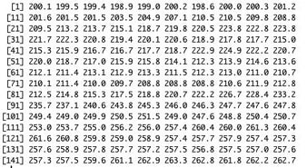
That's telling you that your screen printout is starting at vector item number one. If you've got a vector with lots of values so the printout runs across multiple lines, each line will start with a number in brackets, telling you which vector item number that particular line is starting with. (See the screen shot, below.)

As mentioned earlier, if you want to mix numbers and strings or numbers and TRUE/FALSE types, you need a list. (If you don't create a list, you may be unpleasantly surprised that your variable containing (3, 8, “small”) was turned into a vector of characters (“3”, “8”, “small”).)

And by the way, R assumes that 3 is the same class as 3.0 — numeric (i.e., with a decimal point). If you want the integer 3, you need to signify it as 3L or with the as.integer() function. In a situation where this matters to you, you can check what type of number you've got by using the class() function:

class(3)

class(3.0)

class(3L)

class(as.integer(3))

There are several as() functions for converting one data type to another, including as.character(), as.list() and as.data.frame().

R also has special data types types that are of particular interest when analyzing data, such as matrices and data frames. A matrix has rows and columns; you can find a matrix dimension with dim() such as

dim(my_matrix)

A matrix needs to have all the same data type in every column, such as numbers everywhere.

Data frames are much more commonly used. They're similar to matrices except one column can have a different data type from another column, and each column must have a name. If you've got data in a format that might work well as a database table (or well-formed spreadsheet table), it will also probably work well as an R data frame.

Unlike in Python, where this two-dimensional data type requires an add-on package (pandas), data frames are built into R. There are packages that extend the basic capabilities of R data frames, though. One, the tibble tidyverse package, creates basic data frames with some extra features. Another, data.table, is designed for blazing speed when handling large data sets. It's adds a lot of functionality right within brackets of the data table object 

mydt[code to filter columns, code to create new columns, code to group data]

A lot of data.table will feel familiar to you if you know SQL. For more on data.table, check out the package website or this intro video:

When working with a basic data frame, you can think of each row as similar to a database record and each column like a database field. There are lots of useful functions you can apply to data frames, such as base R's summary() and the dplyr package's glimpse().

Back to base R quirks: There are several ways to find an object's underlying data type, but not all of them return the same value. For example, class() and str() will return data.frame on a data frame object, but mode() returns the more generic list.

If you'd like to learn more details about data types in R, you can watch this video lecture by Roger Peng, associate professor of biostatistics at the Johns Hopkins Bloomberg School of Public Health:

One more useful concept to wrap up this section — hang in there, we're almost done: factors. These represent categories in your data. So, if you've got a data frame with employees, their department and their salaries, salaries would be numerical data and employees would be characters (strings in many other languages); but you might want department to be a factor — ia category you may want to group or model your data by. Factors can be unordered, such as department, or ordered, such as “poor,” “fair,” “good,” and “excellent.”

R command line differs from the Unix shell

When you start working in the R environment, it looks quite similar to a Unix shell. In fact, some R command-line actions behave as you'd expect if you come from a Unix environment, but others don't.

Want to cycle through your last few commands? The up arrow works in R just as it does in Unix — keep hitting it to see prior commands.

The list function, ls(), will give you a list, but not of files as in Unix. Rather, it will provide a list of objects in your current R session.

Want to see your current working directory? pwd, which you'd use in Unix, just throws an error; what you want is getwd().

rm(my_variable) will delete a variable from your current session.