
Google Sheets lets you design spreadsheets with sophisticated features, and one of the most useful to know is dropdown lists. You can add a dropdown list to a cell (or to a range of cells), and when you or another person with access to your spreadsheet clicks the cell, a dropdown will open that shows a list of numbers or words that they can select. The number or word that’s selected will then appear inside the cell.
Some use case examples:
- You need co-workers to enter very specific numbers or words into your spreadsheet. Providing dropdown lists makes this more convenient for them and eliminates the risk of mistyped entries.
- You add a dropdown list containing number presets that immediately change a chart embedded on your spreadsheet.
- You create a spreadsheet to track a project, in which co-workers select their work progress status from a dropdown list.
You can create two kinds of dropdown lists in Google Sheets: The first lists specific numbers or words that you’ve entered as preset choices, while the second lists data that currently appears in a range of cells in your spreadsheet. This guide walks you through the basic steps of creating both types of dropdowns and adding color to them.
Create a dropdown that lists specific numbers or words
Select the cell or the range of cells where you want the dropdown to be on your spreadsheet. Then on the toolbar above your spreadsheet, click Data > Data validation.
On the “Data validation” panel that opens, click List from a range next to “Criteria.” From the menu that opens, select List of items.
 IDG
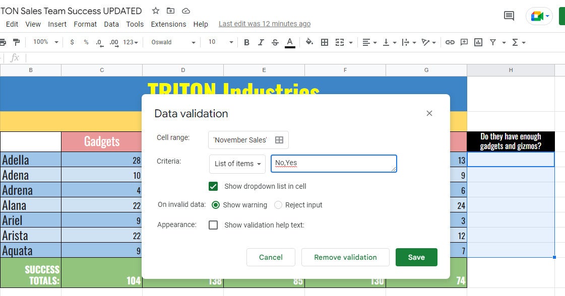
IDGType in the items you want to appear in the dropdown list, separated by commas. (Click image to enlarge it.)
Now, in the box to the right of “List of items,” type in the numbers or words that you want your dropdown list to have. Be sure to separate each number or word with a comma – but don’t type in a space between the numbers or words.
When you create a dropdown list, the cell that it’s in will be marked with a small down arrow. If you don’t want this arrow to appear in the cell, uncheck Show dropdown list in cell.
When you’re finished, click Save on the lower right of the panel.
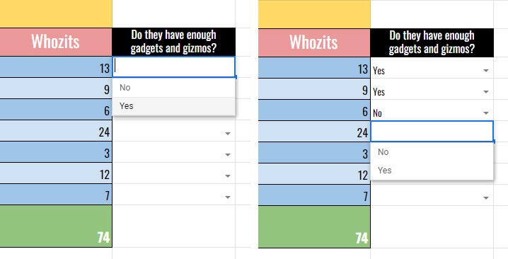
Now when you double-click this cell (or click the down arrow inside it), a dropdown list will open that shows the numbers or words that you typed in above. When you select one of these numbers or words, it will then appear inside the cell.
 IDG
IDGIn the spreadsheet, click the down arrow in a cell with a dropdown list to see the available options (left); the item you select will appear in the cell (right). (Click image to enlarge it.)
Create a dropdown that lists data from your spreadsheet
Select the cell or the range of cells where you want the dropdown to be on your spreadsheet. Then on the toolbar above your spreadsheet, click Data > Data validation.
On the “Data validation” panel that opens, leave the “Criteria” dropdown set to List from a range. In the box to its right, type in the range of cells that you want to appear in the dropdown list. For example: If you type in A1:A10, the data in cells A1 to A10 of your spreadsheet will appear as ten items in the dropdown list.
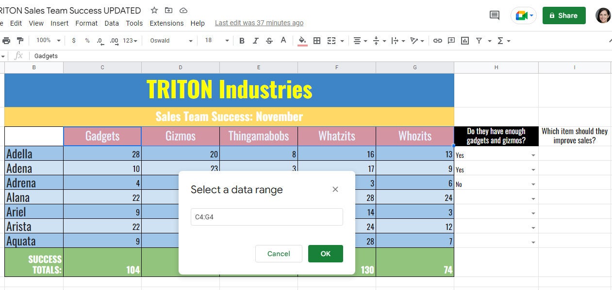
If you click the grid icon that’s inside this entry box, a small panel (“Select a range”) will open over your spreadsheet. With this panel open, you can scroll through your spreadsheet. When you click to select a range of cells, their letter-number designations will appear in this panel’s entry box. Click OK and your selected range of cells will appear in the entry box to the right of “List from a range.”
 IDG
IDGSelect the range of cells whose data you want to appear in the dropdown list. (Click image to enlarge it.)
When you’re finished designating a range of cells, click Save on the lower right of the “Data validation” panel.
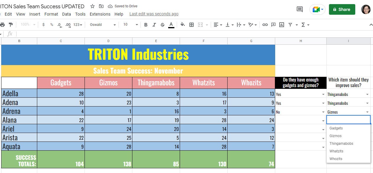
Now when you double-click this cell (or click the down arrow inside it), a list will open that shows the current data in the range of cells that you selected. When you select one of these numbers or words, it will then appear inside the cell.
 IDG
IDGThe dropdown shows a list of items that are currently in the range of cells you selected. (Click image to enlarge it.)
If the range of cells you selected contains formulas, the current number appearing in a cell that’s calculated by a formula will appear in the dropdown list. If the range of cells you selected contains words, those words will appear in the dropdown list. You can even select a range of cells that’s a mix of numbers, words, and formulas. The dropdown will list whatever is currently in each cell in the range of cells that you selected.
Edit or remove a dropdown
Select the cell (or cells) that contains the dropdown list. Then, from the toolbar above your spreadsheet, click Data > Data validation.
On the “Data validation” panel, you can edit the list of numbers or words to the right of “List of items” or change the range of source cells next to “List from a range.”
Or, to remove the dropdown list from the cell or cells, click Remove validation at the bottom of the panel.
Add colors to a dropdown
You’ve created your dropdown list. Now you can assign a color to each item on the list so that when you select one of the items, the text or background of the cell it’s added to turns that color. This can help make your spreadsheet more visually interesting, signify the importance of an item on the list, or emphasize where the item falls in a range.
Assign background colors to items in your dropdown
Click to select the cell that contains the dropdown list. Then, on the toolbar above your spreadsheet, click Format > Conditional formatting. A sidebar (“Conditional format rules”) will open along the right.
 IDG
IDGUse the “Conditional format rules” sidebar to assign colors to your dropdown list. (Click image to enlarge it.)
In the sidebar under the “Format rules” header, click the box with the words Is not empty. From the dropdown list that opens, select Text is exactly.
An entry box with the words “Value or Formula” appears. Type in the entire number or word from your dropdown list that you want to assign a background color.
Next, below the bar labeled “Default,” click the Fill color icon (a paint can). A color selection panel will open. Click to select a color.
 IDG
IDGDesignate the formatting rules, text, and fill color for an item in your dropdown. (Click image to enlarge it.)
Finally, click the Done button.
Now when you select this item from the dropdown list, the background color of this cell will change to the one that you had selected above. When you select another item on this list, the background color will return to the default color.
 IDG
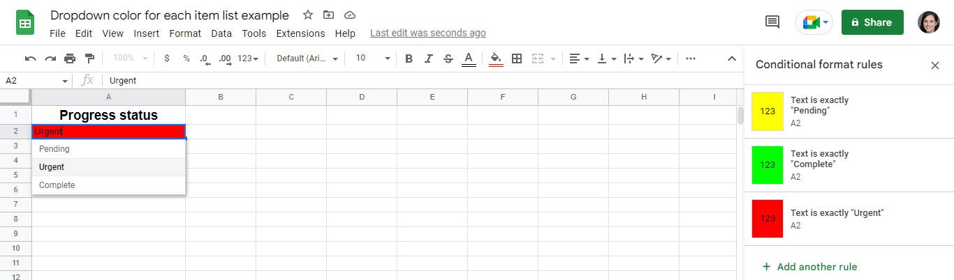
IDGIf you select Pending from the dropdown in the example spreadsheet, its background will be yellow. (Click image to enlarge it.)
To assign a background color for the other items on this cell’s dropdown list, click Add another rule in the “Conditional format rules” sidebar, then repeat the above steps.
 IDG
IDGNow all three dropdown menu choices have an appropriate background color. (Click image to enlarge it.)
Once you grasp how the above works, you can assign different colors to specific numbers that may show up when a formula in your dropdown list calculates them. For example, if the formula for an item in your dropdown list calculates the number 90, then the cell background color could become green when this item is selected from the dropdown list. If the number becomes 20, then the cell background color could become red.
To do this: Following the steps above, type in 90 and then assign the color green to it. Then, in the “Conditional format rules” panel, click Add another rule. Follow the steps above again, type in 20, and assign it the color red.
Assign text colors to items in your dropdown
You can assign the items in your dropdown list text colors instead of or in addition background colors. Follow the steps above, and in the “Formatting style” area of the “Conditional format rules” sidebar, click the Text color icon (a capital “A”) and choose a color. Click the Fill color icon and choose a background color or click None.
Assign a color scale to items in your dropdown
You can assign a range of background colors to the items in your dropdown list. For example, you could set it so that if the user selects 100 from your dropdown list, the cell background color turns green. For 60, the cell background turns yellow. For 10, the cell background turns red. And for any numbers on your dropdown list that fall between two of these three, the background will appear as an intermediate shade between the two colors.
To illustrate this, let’s create a dropdown list that contains ten numbers (10, 20, 30, etc.) that can be selected.
Click to select the cell that contains the dropdown list. Then on the toolbar above your spreadsheet, click Format > Conditional formatting to open the “Conditional format rules” sidebar along the right.
On this sidebar, click the Color scale tab on the upper right. The sidebar will switch to the “Color scale” panel.
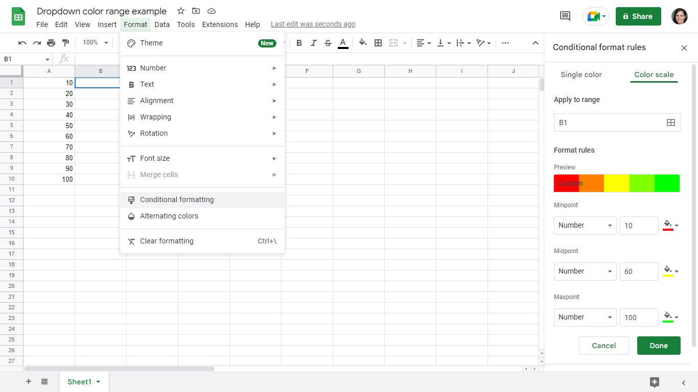
Next, under the “Format rules” heading, click Minpoint to open its dropdown menu. For our example, select Number. Type 10 In in the entry box to the right.
 IDG
IDGTo set up a color range, assign a Minpoint, Midpoint, and Maxpoint value and color. (Click image to enlarge it.)
Click the paint can icon to the right. From the color selection panel that opens, click to select the color red.
Select Number from the dropdown lists for Midpoint and Maxpoint, too, and type in 60 and 100 respectively. Click their paint can icons, and select the color yellow for Midpoint and green for Maxpoint. As you set these points and colors, you’ll see a preview of the whole color range just above.
Click the Done button.
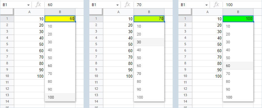
Now when the number 60 is selected from the dropdown list, the cell’s background color turns to yellow. When you select 70, the background color turns to a yellow that has a tinge of green mixed in. When you select 100, the cell’s background color will be fully green.
 IDG
IDGUsing a color scale provides a visual indicator for the values of items in a dropdown list. (Click image to enlarge it.)
Manage the colors of items in your dropdown
If you want to change the text or background colors you’ve assigned to the items in a dropdown list, click to select the cell that contains the dropdown list, then click Format > Conditional formatting to open the “Conditional format rules” sidebar. In the sidebar you’ll see a list of the color assignments you’ve made for the dropdown list, each with its own color swatch.
Remove a color: Move the pointer over the color swatch and click the trashcan icon that appears to the right of the swatch.
 IDG
IDGClick the trashcan to remove a color assignment.
Change a color: Click the color swatch. If it’s a single color, the sidebar will switch to the “Single color” panel. If it’s a range of colors, the sidebar will switch to the “Scale color” panel. Click the paint can icons on either panel to change colors.
Add a new color: Click Add another rule. The sidebar will switch to the “Single color” panel. If you want to assign a range of colors to the items in your dropdown list, click Scale color on the upper right to switch to this panel.
Read this next: Google Sheets power tips: How to use filters and slicers