
One of the most commonly used Microsoft programs, Excel is highly useful for data collecting, processing, and analysis. To fully harness Excel’s powers, though, you need to make use of formulas.
Excel formulas allow you to perform calculations, analyze data, and return results quickly and accurately. The usefulness of formulas is even greater once you start dealing with large data sets. With the correct formula, Excel can process vast amounts of information in a matter of seconds.
What is a formula in Excel?
A formula is an expression that operates on values in a range of cells in Excel. Using formulas, you can perform calculations and data analysis on the contents of the cells. Formulas can be as simple as adding a column of numbers together or as complex as returning the kurtosis of a data set. They can be incredibly useful when you want to turn spreadsheet data into meaningful information for driving business decisions.
What is a function in Excel?
A function is a built-in formula in Excel — basically, a shortcut for performing a calculation or other operation on cell data. There are nearly 500 Excel functions, and the list continues to grow every year. Fortunately, most of the actions that a typical business user would want to perform can be done with just a handful of functions.
In this article we’ll look at five useful types of formulas and functions that will get you started performing data analysis in Excel. Along the way, you’ll learn several different ways to enter formulas and functions in Excel.
We’ll demonstrate using Excel for Windows under a Microsoft 365 subscription. If you’re using a different version of Excel, you might not have exactly the same interface and options, but the formulas and functions work the same.
1. Basic mathematics formulas and functions
We’re going to group these formulas together since they are very simple and have similar syntax. All formulas in Excel start with the equal sign (=) and build from there.
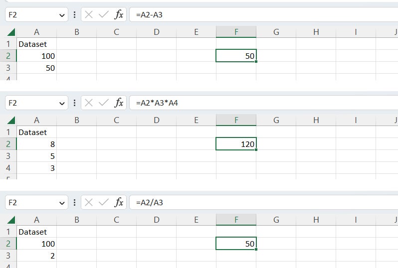
Adding, subtracting, multiplying, and dividing
To add the numbers in two cells together, first click the on the target cell where you want the total to appear. Then type = in the cell to start the formula.
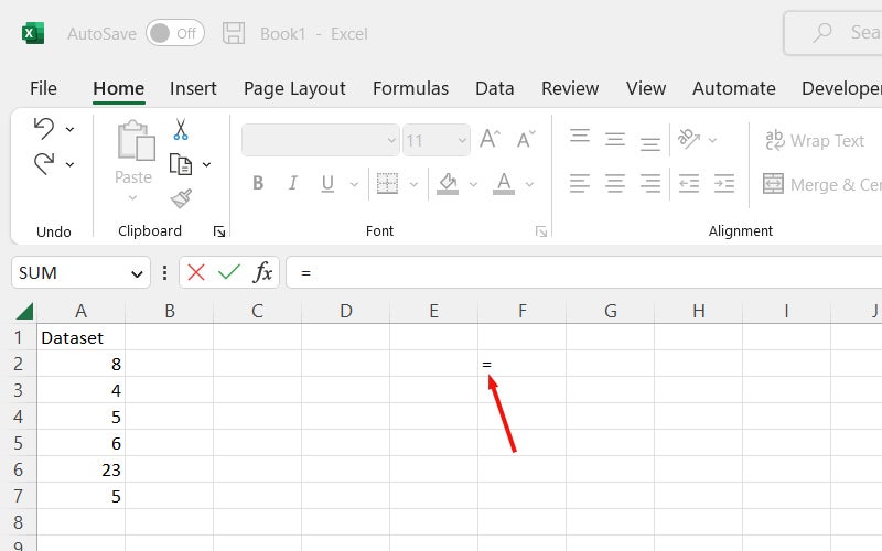 Shimon Brathwaite / IDG
Starting a formula in Excel.
Next, click on the cell that contains the first number you want to add, and its cell reference (such as A2) will appear next to the equal sign in the formula.
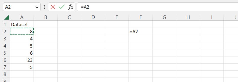 Shimon Brathwaite / IDG
When you select a cell when building a formula, its cell reference appears in the formula.
Type + next to the first cell reference. Then click the cell that contains the second number you want to add, and its cell reference (such as A3) will appear next to the + sign. The full syntax for the formula to add the values in cells A2 and A3 is:
=A2+A3
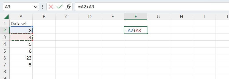 Shimon Brathwaite / IDG
The complete addition formula appears in both the target cell and the formula bar above.
Note that in addition to appearing in the target cell, the formula also appears in the formula bar directly above the worksheet. Once you’ve inserted the initial = sign in the target cell, you can type your formula in the formula bar. It’s sometimes easier to see the whole formula and work with it in the formula bar than down in the worksheet page.
If you wanted to add additional numbers to your total, you’d type another + sign, select another cell, and so on. Once your formula is complete, press Enter, and the result appears in the target cell.
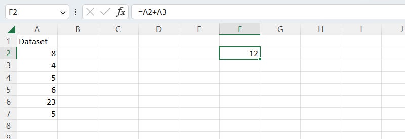 Shimon Brathwaite / IDG
Press Enter, and the result appears in the target cell.
Subtraction, multiplication, and division calculations work the same way. You simply change the operator — the symbol that tells Excel what math operation you want to perform — from the + sign to the – sign for subtraction, the * sign for multiplication, or the / sign for division.
 Shimon Brathwaite / IDG
Subtraction, multiplication, and division actions. The formula for each is shown in the formula bar; the result in the target cell.
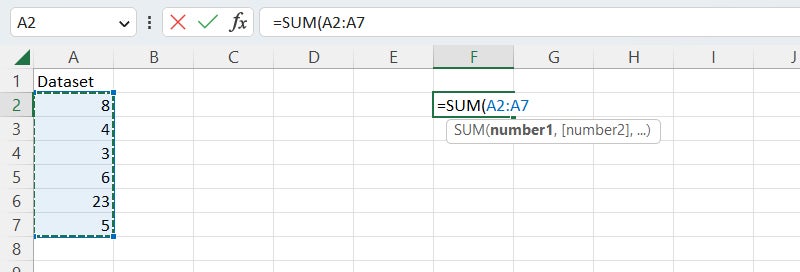
Adding numbers with the SUM function
There’s a quicker way to add together a group of numbers. This is where Excel’s built-in SUM function comes in.
First click on the target cell where you want the total to appear. Then type =SUM to start the function. A list of options will come up. Click the first option, SUM. You’ll now see =SUM( in the target cell.
 Shimon Brathwaite / IDG
Starting a SUM function.
Just underneath the cell with the SUM function is a tooltip showing the SUM syntax:
=SUM(number 1, [number2],…)
To add individual cells together, select a cell, type a comma, select another cell, and so on. (Alternatively, you can type a cell reference, type a comma, type another cell reference, and so on.)
If you want to add consecutive cells (such as in a row or column), select the first cell, then hold down the Shift key and select the final cell in the group. (Or you can type in the cell references for the first and last cells separated by a colon — for instance, A2:A7 selects A2, A7, and all the cells in between.)
 Shimon Brathwaite / IDG
Select the range of cells you want to add together.
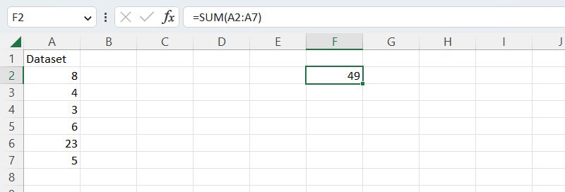
Once all the cells you want to add together are selected, hit Enter.
Now you should see the final result, which is the sum of the numbers you highlighted. If you highlight that target cell again, you’ll see the full formula in the formula bar — in our example, it’s:
=SUM(A2:A7)
 Shimon Brathwaite / IDG
The SUM function is shown in the formula bar; the result appears in the target cell.
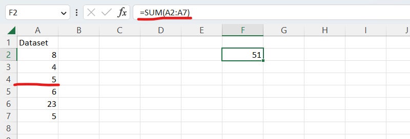
One important thing to note for all Excel formulas is that they produce relative values. This simply means that if any of the values in the selected cells changes, then the final number will change to reflect that.
 Shimon Brathwaite / IDG
If the value of a cell used in a formula changes, the result also changes.
If you want to make it an absolute value, a number that will not change even if the cells that were used to calculate it change, then you need to right-click the cell and select Copy from the pop-up menu. Then right-click the cell again and, under Paste Options, select the Values button (the icon of a clipboard with 123).
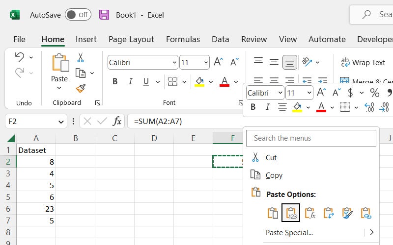 Shimon Brathwaite / IDG
Copy and paste the value into the cell to prevent the value from changing if one of the source cell’s values changes.
Now when you select that cell you’ll just see the plain number, not a formula, in the formula bar.
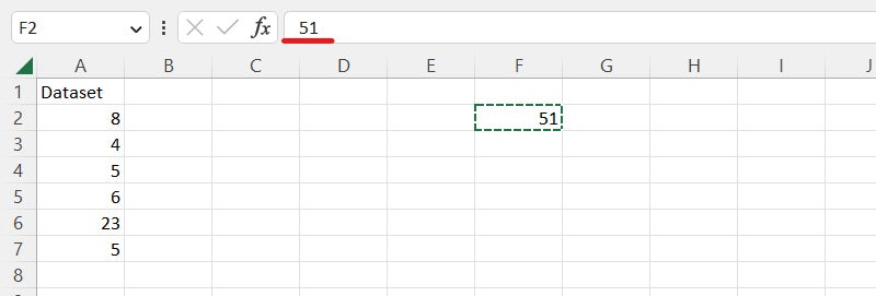 Shimon Brathwaite / IDG
The cell now contains an absolute value, not a formula.
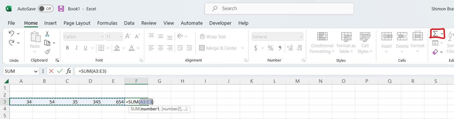
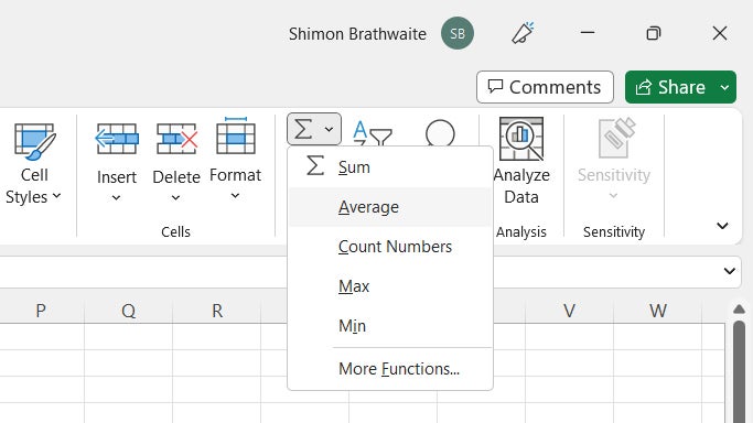
Tip: Excel provides a SUM shortcut in certain circumstances. If you have a series of numbers in a row or a column, Excel assumes you want to add them together. So if you place your cursor in the cell to the right of a row of numbers and click the AutoSum button toward the right end of the Ribbon’s home tab, Excel automatically selects the numbers in the row, then adds them together when you press Enter. Likewise, if you place your cursor in the cell below a column of numbers, click AutoSum, and hit Enter, Excel totals up the numbers in the column.
 Shimon Brathwaite / IDG
AutoSum is a shortcut for adding a row or column of numbers. (Click image to enlarge it.)
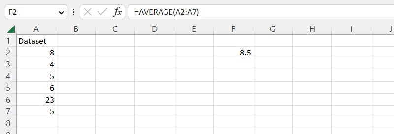
Calculating the average with the AVERAGE function
To calculate the average of a group of numbers, repeat the same steps but using the syntax =AVERAGE and highlighting the cells containing the numbers that you want to use in the calculation.
 Shimon Brathwaite / IDG
To quickly calculate the average of a group of numbers, use the AVERAGE function.
Tip: As with SUM, there’s a shortcut for using the AVERAGE function if you have a series of numbers in a row or a column. Place your cursor in the cell to the right of a row of numbers or in the cell below a column of numbers. Click the tiny down arrow at the right side of the AutoSum button, select Average from the menu that appears, and hit Enter. Excel calculates the average of the values in that row or column.
 Shimon Brathwaite / IDG
There’s an AutoSum shortcut for the AVERAGE function as well.
Find more details, examples, and best practices for these functions at Microsoft’s SUM function and AVERAGE function support pages.
2. The IF function
This function helps you automate the decision-making process by applying if-then logic to your data. Using this function, you can have Excel perform a calculation or display a certain value depending on the outcome of a logical test. For example, you can create a test that checks if the value of a cell is greater than or equal to the value of 18 and enter “Yes” or “No” accordingly.
While we’re learning this function, we’ll cover another way to enter functions in Excel: by using the Formulas tab on the Ribbon. Here you’ll find buttons that provide quick access to functions by category: AutoSum, Financial, Logical, Text, Date & Time, and so on. Being able to browse through functions by category can be helpful if you can’t remember the exact name of a function or aren’t sure how to spell it.
To enter the IF function, select the target cell, and on the Formulas tab, click the Logical button, then select IF from the list of functions that appears.
Alternatively, you can click the Insert Function button all the way to the left of the Formulas tab. An “Insert Function” pane appears, showing a list of commonly used functions.
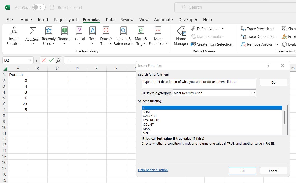 Shimon Brathwaite / IDG
Instead of typing = to start a function, you can go to the Formulas tab and select Insert Function. (Click image to enlarge it.)
Select IF from the list and click OK. (If the function you want isn’t in the “Commonly Used” list, select a different category or All to see all available functions.)
The Function Arguments pane appears, and you’ll see =IF() in the target cell.
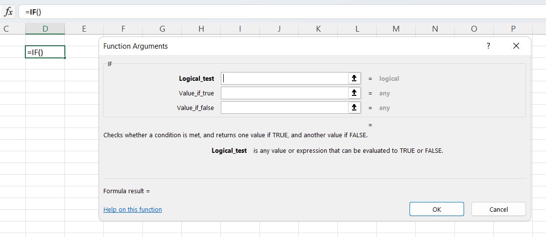 Shimon Brathwaite / IDG
You can use the Function Arguments pane to build a function. (Click image to enlarge it.)
The IF function syntax is as follows:
=IF(logical_test,”value_if_true”,”value_if_false”)
You’ll notice that the Function Arguments pane for the IF function has fields for Logical_test, Value_if_true, and Value_if_false. In our “greater than or equal to 18” example, the logical test is whether the number in the selected cell is greater than or equal to 18, the value if true is “Yes,” and the value if false is “No.” So we’d enter the following items in the pane’s fields like so:
Logical_test: B2>=18
Value_if_true: “Yes”
Value_if_false: “No”
or just type the full formula into the target cell:
=IF(B2>=18,”Yes”,”No”)
This tells Excel that if the value of cell B2 is greater than or equal to 18, it should enter “Yes” in the target cell. If the value of cell B2 is less than 18, it should enter “No.”
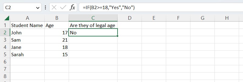 Shimon Brathwaite / IDG
The IF function in action.
Tip: When using functions like this, rather than entering the function repeatedly for each row, you can simply click and drag the tiny square on the bottom right of the cell that contains the function. Doing so will autofill each of the rows with the formula, and Excel will change your cell references to match. For example, when the formula we used in cell C2 that references cell B2 is autofilled into cell C3, it changes to reference cell B3 automatically.
 Shimon Brathwaite / IDG
Autofilling a formula to subsequent rows in the column.
Find more details at Microsoft’s IF function support page.
Next page: SUMIF, COUNTIF, CONCAT, and VLOOKUP →